null hypothesis and p-value Link to heading

very useful post

so to summarize somewhat into my own words:

1. null hypothesis is

The null hypothesis, H0 is the commonly accepted fact; it is the opposite of the alternate hypothesis. Researchers work to reject, nullify or disprove the null hypothesis.

this is coming from here

so how do we “nullify” the hypothesis? we are using p-value

2. we are using p-value to nullify the hypothesis

the common chose p-value is 0.05, if the calculated p-value is less than 0.05, then it’s nullified; otherwise, the hypothesis stays.

Regression - [Supervised Learninng] Link to heading

Regression is a useful tool to predict a continuous number.

Linear Regression Link to heading

Before building a linear regression model, there is a caveat

Assumptions of Linear Regression:

1. linearity
2. homoscedasticity
3. multivariate nomarlity
4. independence of errors
5. lack of multicollinearity

Dummy variable trap for linear regression Link to heading

take an example here, say we have a model like this y = b0 + b1*x1 + b2*x2 + b3*x3, and we have one more column we want to take into consideration, say it’s state.

we have two distinct states inside the column, they are “New York” and “California”. by encoding, we can say it it’s NY, we will have a vector like [1, 0], so for CA, we will have [0, 1]. just a representation.

so, it comes to an question that how should we include them, is it y = b0 + b1*x1 + b2*x2 + b3*x3 + b4*D1 or is it y = b0 + b1*x1 + b2*x2 + b3*x3 + b4*D1 + b5*D2?

the answer is the first one y = b0 + b1*x1 + b2*x2 + b3*x3 + b4*D1.

the reason is that, we know state is mutual exclusive, meaning it couldn’t be both NY and CA, so naturally D1+D2 = 1. so if we introduce both D1 and D2 in the function we will violate “lack of multicollinearity” assumption.

Linear Regression template Link to heading

1. import the libraries
2. import the dataset
3. encoding categorical data: hot-encoding will always come to the first columns
4. splitting the dataset into training set and test set
5. training the linear regression model on training set
6. predict the test dataset result

Backward Elimination Link to heading

the following code snippet copied from machine learnin a-z

import statsmodels.formula.api as sm
def backwardElimination(x, sl):
    numVars = len(x[0])
    for i in range(0, numVars):
        regressor_OLS = sm.OLS(y, x).fit()
        maxVar = max(regressor_OLS.pvalues).astype(float)
        if maxVar > sl:
            for j in range(0, numVars - i):
                if (regressor_OLS.pvalues[j].astype(float) == maxVar):
                    x = np.delete(x, j, 1)
    regressor_OLS.summary()

    return x

SVR Link to heading

SVR vs SVM, both have support vector in the names, but they are for different purposes.

SVR stands for support vector regression, in essence it’s a regression algorithm, SVR will works forr continuous values

whereas SVM is a classification algorithm.

As name indicated, SVR could be used to predict.

template for SVR:

1. import libs
2. import dataset
3. feature scaling
4. train the SVR model on the whole dataset
5. predict new result
6. visualize the result

Noted number 3. why do a feature scaling? Because in machine learning algorithms, it’s essential to calculate distance between data. If not scale, the feature with higher value range starts dominating. check details here

And remember to call inverse_transfrom method after you got the predictions. Make sure to use the right scaler.

Decision Tree Regression Link to heading

Decision tree can be used to both regression and classification.

The essence of decision tree regression is to split the tree, calculate the entropy for each leaf node in order to find the most important attribute.

So, that said, we don’t need to do feature scaling on decision tree model.

Noted that decision tree regression is not suitable for single feature model(?), it will perform better for multi feature model.

The same for random forest regression, no feature scaling

Random Forest and Ensemble Learning Link to heading

Random forest is one kind of ensemble learning. The essence of ensemble learning, random forest specifically in our case, is to enlarge the hypothesis, and combine hypotheses later on.

Random forest seems more adaptable on classification because by utilizing the essence of ensemble learning, we hope it will decrease the classification: it will be unlikely for all 5 hypotheses to misclassify than one; in other word, we are more safe to trust the all 5 “misclassifies”

R-Squared (R^2) - performation of the regression model Link to heading

Simple definition of R squared.

SS res = SUM(yi - y^i)^2 SS tot = SUM(yi - yavg)^2

R^2 = 1-SS res/SS tot

R^2 ideally would be from 0 to 1, the more to 1 the better, the more to 1 the more fit to the data.

Adjusted R Squared

The intuition that we have an adjusted R squared is that because it (original R squared) will never decrease if add more feature into the hypothesis

Adj R^2 = 1-(1-R^2)(n-1)/(n-p-1_)

where p - number of regressors and n - sample size

R squared is also a criteria to choose which model to use.

Classification - [Unsupervised Learning] Link to heading

Classification is a powerful tool to predict a category.

Logistic Regression Link to heading

Logistic regression template

1. import libs
2. import dataset
3. splitting the dataset into training and test set
4. feature scaling
5. training (fit) the logistic regression model on training dataset
6. predict a new result
7. predicting the test set result
8. making the confusion matrix
9. visualize both train and test set results

1-4 are data preprocessing, 5 is fit step, 6,7 are prediciton and rest are visualization.

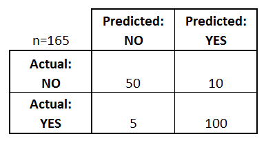
Confusion matrix and accuracy score Link to heading

In sklearn.metrics, but what is underneath?

A confusion matrix is a table that is often used to describe the performance of a classification model (or “classifier”) on a set of test data for which the true values are known.

please go to dataschool

K Nearest Neighbor Link to heading

SVM Link to heading

back to SVR, in stead of using it to predict continous numbers, we use it to classify.

Some terms:

• hyperplane
• support vectors
• maximum margin

SVM is somewhat special because the support vectors it uses to construct margin are the “edge cases”. Poeple find it predicts better than non SVM algo often because it uses the edge cases.

Kernel SVM Link to heading

If the data is linearly separable, then use linear SVM; otherwise, we cannot use linear SVM.

Then the question becomes what to use?

Some intuition that classify some non linear dataset using SVM is to make dataset to a higher dimension.

The pros of doing that is it sometimes is easy to find the hyperplane when in a higher dimension; the cons is computing intensive.

After using SVM solving it in a higher dimension, then map it back.

Now, after the intuition, how do we actually do it?

Since we are under Kernel Function, yes, by applying kernel functions, basically we are doing those.

An example here. In the middle of the post, it generates a nice graph. First using kernel function in this case RBF pull data from 2d to 3d, classify them, and then push back data from 3d to 2d. Contour will be left on 2d plate. (kernel trick???)

Some common kernel functions that we might use including:

• Gaussian RBF
• Polynomial kernel function
• Sigmoid kernel function

Kernel Tricks Link to heading

According to this post, keneral trick is so important that it bridges linearity to non-linearity.

Non linear SVR (not SVM) Link to heading

By using kernel trick, or pull data into higher demensions-find max and min hyperplane-push higher demension back to original, we could find a tube (in this time it’s a curved cube instead of two lines)

How do we do that? Kernel tricks. So kernel tricks is very important.

Naive Bayes Link to heading

The following is the Bayes Thereom

\( {P(A|B)}{P(B)} = {P(B|A)}{P(A)}\)

Naive Bayes Classifier intuition Link to heading

Plan to attack a problem, have to borrow Bayes Thereom again

\( {P(A|B)} = \frac{P(B|A)*P(A)}{P(B)} \)

We are now giving each element a new name:

1. \( {P(A)} \), the Prior Probablility
2. \( {P(B)} \), the Marginal Likelihood
3. \( {P(B|A)} \), the Likelihood
4. \( {P(A|B)} \), the Posterior Probablility

When attack a problem, we want to calculate elements in order.

A concrete example, we assign B as the features dataset X, and given X, we have multiple categories that can classify to; in other words, A can assign to cat1, cat2, etc.

So the function now becomes:

\( {P(cat1|X)} = \frac{P(X|cat1)*P(cat1)}{P(X)} \)

If we want to predict a data point, x, we need to calculate all \( {P(cat1|X)} \) and \( {P(cat2|X)} \), at last compare them and assign to the correct cat

Noted for number2, the marginal likelihood. Calculating that likelihood will introduce a “margin”, which will be having the similar features of the “newly added point/the point to be predicted”. So feels like choosing that “margin” is an critical work during the calulation.

Decision Tree Classification Link to heading

Classification and Regression Trees (CART)

Decision Tree recently was dying, but some other algorithm utilize the simplicity of the decision trees to make it reborn.

They are Random Forest, Gradient Boosting, etc.

Random Forest Classification Link to heading

Random Forest is some kind of ensemble learning.

Evaluation of classification Link to heading

• confusion matrix: In general, false positive is more like a warning, whereas false negative is like the real “error”. In diagnal, they are the right prediction.
• Cumulative Accuracy Profile (CAP) vs. Receiver Operating Characteristic (ROC)
  • some explains
  • when doing cap analysis, this guy introduce AR 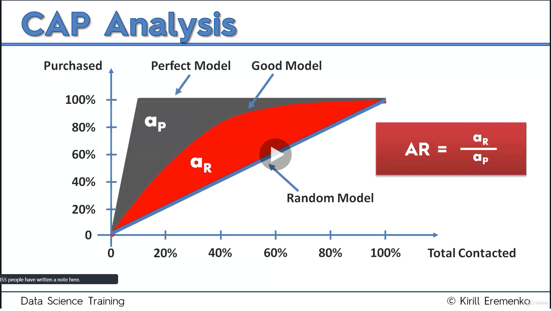and some criteria

Clustering Link to heading

K Means Link to heading

1. choose the number K of clusters
2. select at random K points. the centroids (not necessarily from your dataset)
3. assign each data point to the closest centroid, that forms k clusters (calculate distance to the centroid)
4. compute and place the new centroid of each cluster. (average of data within the cluster)
5. reassign each data point to the new closest centroid.

if any reassignment took place, go to 4 again.

otherwise, the alg is finished.

K means init trap Link to heading

different select of centroids will result in false consequence.

use Kmean++ algorithm.

K Means: choosing the number number of clusters Link to heading

\( WCSS = \sum_{Pi in Cluster j}^{total i} \sum_{j}^{total j} distance(Pi, Cj)^2 \)

WCSS will be decreasing continously and to 0 if every point has a centroid of its own.

What should we do to optimize it? Draw WCSS vs Number of Clusters and using elbow method to decide the number of clusters.

K Mean Procedures Link to heading

1. import libs
2. import datasets
3. elbow method to find number of clusters
4. train the K Means model on the dataset
5. visualization

Hierarchical Clustering Link to heading

We majorly focus on the agglomerative clustering rather than divisive here

1. Make each data point a single-point cluster -> forms N clusters
2. take the two closest clusters and make them one cluster
3. repeat until there is only one cluster

How to define the distance between the two clusters?

There are several options: 1. closest points, 2. furthest points, 3. average distance, 4. distance between centoids. As long as it is consistent, then it’s fine

How to decide the best cluster numbers?

Dendrograms Link to heading

what is a dendrogram

And the quickest way making a decision is to see which vertical line between the two horizontal line is the longest.

like this example below

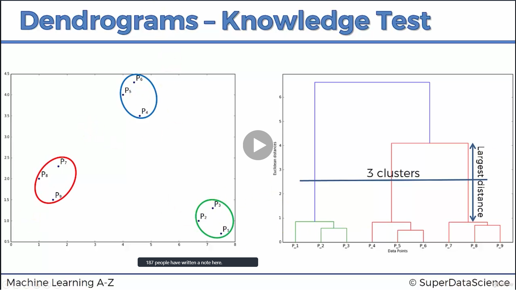
we see the correct answer for this is 3 clusters, not 2 clusters because the red line has the largest distance.

Association Rule Learning Link to heading

Apriori Link to heading

\( {lift(M_1 -> M_2)} = \frac{confidence(M_1 -> M_2)}{support(M_2)} \)

A practical usage of this alg would be frequent purchased together. (I am guessings)

Eclat Link to heading

Only support matters. Still use apriori model to give rules, but using eclat method to analyze.

Reinforcement Learning Link to heading

What is reinforcement learning?

Reinforcement Learning is a subset of machine learning. It enables an agent to learn through the consequences of actions in a specific environment. It can be used to teach a robot new tricks, for example. – towardsdatascience.com

Summary of UCB and Thompson Sampling Link to heading

• UCB is a deterministic algorithm whereas Thompson Sampling is a probalistic algorithm.

Upper Confidence Bound Link to heading

Coming from multi-armed bandit problem.

Some simplified steps for UCB alg:

1. At each round n, we consider two numbers for each ad i:
   • \( N_i(n) \) - the number of times the ad i was selected up to round n
   • \( R_i(n) \) - the sum of rewards of the ad i up to round n
2. From these two numbers we compute:
   • the average reward of ad i up to round n \( \bar{r}_i(n) = \frac{R_i(n)}{N_i(n)} \)
   • the confidence interval \( [\bar{r}_i(n) - \Delta_i(n), \bar{r}_i(n) + \Delta_i(n)] \) at round n with \( \Delta_i(n) = \sqrt{\frac{3log(n)}{2N_i(n)}} \)
3. We select the ad i that has the maximum UCB \( \bar{r}_i(n) + \Delta_i(n) \)

Thompson Sampling Link to heading

some simplified steps for Thompson Sampling

1. At each round n, we consider two numbers for each ad i:
   • \( N_i^1(n) \) - the number of times the ad i got reward 1 up to round n.
   • \( N_i^0(n) \) - the number of times the ad i got reward 0 up to round n.
2. For each ad i, we take a random draw from the distribution \( \theta_i(n) = \beta(N_i^1(n)+1, N_i^0(n)+1) \)
3. We select the ad that has the highest \( \theta_i(n) \)

NLP Link to heading

Types of Natural Language Processing Link to heading

Once there were classic NLP, and there were deep learning.

Now we have the intersection called DNLP, within that intersection, we have seq2seq

TLDR: classic NLP DNLP(including seq2seq) Deep Learning

Classical v.s. deep learning models Link to heading

• classical examples:
  • if/else rules used to be used on chatbot
  • some audio frequency analysis
  • bag of words used for classification
• not so classical –> deep learning
  • CNN for text recognition used for classification
  • seq2seq can be used for many applications.

Bag of Words Link to heading

The bag-of-words model is a simplifying representation used in natural language processing and information retrieval (IR). – wikipedia

Intuition Link to heading

One specific sentence is represented by a array [0, 0, ..., 0], where array[0] represents the start of the sentence (SOS), array[1] represents the end of the sentence (EOS), array[-1] represents the special words.

Usually array is with length of 20000 elements long.

The number of 20000 is because of

Most adult native test-takers knows ranging from 20000-35000 — The Economist

By feeding training data, some sentences prepared are used to train the model.

Assumptions Link to heading

• position of the words in the document doesn’t matter.

Limitations Link to heading

Limitations on bag of words algorithm is that it can only answer Y/N question.

choice of classifier using bag of words Link to heading

see from here

• No data –> handwritten rules.
• less training data –> naive bayes
• reasonable amount –> SVM & Logical regression. Decision trees maybe.

Neural Network Link to heading

simplified training process Link to heading

1. Randomly initialize the weights to small numbers close to 0 (but not 0)
2. input the first observation of your dataset in the input layer, each feature in one input node.
3. forward-propagation, getting result y.
4. compare the predicted result to the actual result. measure the generated error.
5. back propagation. update the weights according to how much they are responsible for the error. the learning rate decides by how much we update the weights.
6. repeat 1-5 update the weights after each observation (Reinforcement Learning). if update the weigths only after a batch of observations (Batch Learning).
7. When the whole traning set passed thru the ANN, that makes an epoch. Redo more epochs.